41 excel add data labels from different column
Custom Data Labels with Colors and Symbols in Excel Charts - [How To ... Step 3: Turn data labels on if they are not already by going to Chart elements option in design tab under chart tools. Step 4: Click on data labels and it will select the whole series. Don't click again as we need to apply settings on the whole series and not just one data label. Step 4: Go to Label options > Number. Custom data labels in a chart - Get Digital Help Press with mouse on Add Data Labels". Double press with left mouse button on any data label to expand the "Format Data Series" pane. Enable checkbox "Value from cells". A small dialog box prompts for a cell range containing the values you want to use a s data labels. Select the cell range and press with left mouse button on OK button. The chart ...
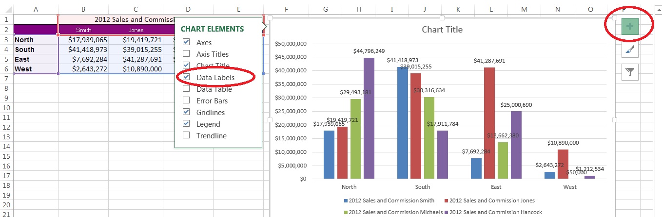
Change the format of data labels in a chart To get there, after adding your data labels, select the data label to format, and then click Chart Elements > Data Labels > More Options. To go to the appropriate area, click one of the four icons ( Fill & Line, Effects, Size & Properties ( Layout & Properties in Outlook or Word), or Label Options) shown here.
Excel add data labels from different column
Excel: Merge tables by matching column data or headers Select any cell within your main table and click the Merge Two Tables button on the Ablebits Data tab: Make sure the add-in got the range right, and click Next: Select the lookup table, and click Next: Specify the column pairs to match, Seller and Product in our case, and click Next: Tip. How to Customize Your Excel Pivot Chart Data Labels - dummies To add data labels, just select the command that corresponds to the location you want. To remove the labels, select the None command. If you want to specify what Excel should use for the data label, choose the More Data Labels Options command from the Data Labels menu. Excel displays the Format Data Labels pane. How to add data labels from different columns in an Excel chart? To add data labels, right-click the set of data in the chart, then pick the Add Data Labels option in Add Data Labels from the context menu. This will bring up a new window. Step 6 This is the data label that is currently shown in the chart. Step 7 If you click any data label, then all data labels will be selected.
Excel add data labels from different column. How to add or move data labels in Excel chart? - ExtendOffice 2. Then click the Chart Elements, and check Data Labels, then you can click the arrow to choose an option about the data labels in the sub menu. See screenshot: In Excel 2010 or 2007. 1. click on the chart to show the Layout tab in the Chart Tools group. See screenshot: 2. Then click Data Labels, and select one type of data labels as you need ... How to create Custom Data Labels in Excel Charts - Efficiency 365 Create the chart as usual. Add default data labels. Click on each unwanted label (using slow double click) and delete it. Select each item where you want the custom label one at a time. Press F2 to move focus to the Formula editing box. Type the equal to sign. Now click on the cell which contains the appropriate label. Multiple Data Labels on bar chart? - Excel Help Forum Select A1:D4 and insert a bar chart. Select 2 series and delete it. Select 2 series, % diff base line, and move to secondary axis. Adjust series 2 data references, Value from B2:D2. Category labels from B4:D4. Apply data labels to series 2 outside end. select outside end data labels and change from Values to Category Name. Dynamically Label Excel Chart Series Lines - My Online Training Hub To modify the axis so the Year and Month labels are nested; right-click the chart > Select Data > Edit the Horizontal (category) Axis Labels > change the 'Axis label range' to include column A. Step 2: Clever Formula The Label Series Data contains a formula that only returns the value for the last row of data.
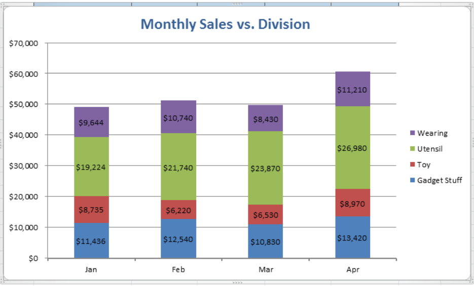
How to Use Cell Values for Excel Chart Labels - How-To Geek Select the chart, choose the "Chart Elements" option, click the "Data Labels" arrow, and then "More Options." Uncheck the "Value" box and check the "Value From Cells" box. Select cells C2:C6 to use for the data label range and then click the "OK" button. The values from these cells are now used for the chart data labels. How to Change Excel Chart Data Labels to Custom Values? - Chandoo.org You can change data labels and point them to different cells using this little trick. First add data labels to the chart (Layout Ribbon > Data Labels) Define the new data label values in a bunch of cells, like this: Now, click on any data label. This will select "all" data labels. Now click once again. Adding Labels to Column Charts | Online Excel Training | Kubicle To add data labels, just right-click on a data series and click add data labels. To see the data labels clearly, I'll need to select them and change their color to white. The data labels are determined by the vertical axis of your chart. Currently, the vertical axis shows millions, therefore, my data labels are shown in millions as well. Add Data Labels From Different Column In An Excel Chart A.docx Click any data label to select all data labels, and then click the specified data label to select it only in the chart. 3. Go to the formula bar, type =, select the corresponding cell in the different column, and press the Enter key. See screenshot: 4. Repeat the above 2 - 3 steps to add data labels from the different column for otherdata points.
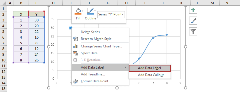
Add or remove data labels in a chart - support.microsoft.com Right-click the data series or data label to display more data for, and then click Format Data Labels. Click Label Options and under Label Contains, select the Values From Cells checkbox. When the Data Label Range dialog box appears, go back to the spreadsheet and select the range for which you want the cell values to display as data labels. How to Add Data Labels to an Excel 2010 Chart - dummies On the Chart Tools Layout tab, click Data Labels→More Data Label Options. The Format Data Labels dialog box appears. You can use the options on the Label Options, Number, Fill, Border Color, Border Styles, Shadow, Glow and Soft Edges, 3-D Format, and Alignment tabs to customize the appearance and position of the data labels. How to add data labels from different column in an Excel chart? This method will guide you to manually add a data label from a cell of different column at a time in an Excel chart. 1. Right click the data series in the chart, and select Add Data Labels > Add Data Labels from the context menu to add data labels. 2. How to Print Labels from Excel - Lifewire Select Mailings > Write & Insert Fields > Update Labels . Once you have the Excel spreadsheet and the Word document set up, you can merge the information and print your labels. Click Finish & Merge in the Finish group on the Mailings tab. Click Edit Individual Documents to preview how your printed labels will appear. Select All > OK .
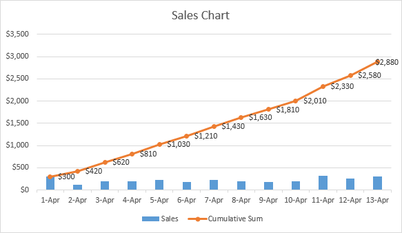
How to do a running total in Excel (Cumulative Sum formula)
How can I add data labels from a third column to a scatterplot? Under Labels, click Data Labels, and then in the upper part of the list, click the data label type that you want. Under Labels, click Data Labels, and then in the lower part of the list, click where you want the data label to appear. Depending on the chart type, some options may not be available.
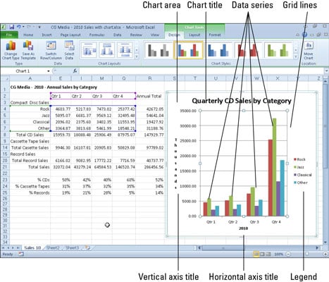
Getting to Know the Parts of an Excel 2010 Chart - dummies
Can I add data labels from an unrelated column to a simple 2-D column ... I would like to add data labels to the vertical chart representations with values from a third column. I am trying to show how many input/data points were included for each displayed column percentage (height) on the chart. The third column values range from 10-200, with an couple outliers up to 5,500, so a third axis doesn't display the data well.
![How to Create One Variable Data Table in Excel 2013 - [What If Analysis]](http://www.exceldemy.com/wp-content/uploads/2014/01/creating-one-variable-data-table.png)
How to Create One Variable Data Table in Excel 2013 - [What If Analysis]
Excel charts: add title, customize chart axis, legend and data labels Click anywhere within your Excel chart, then click the Chart Elements button and check the Axis Titles box. If you want to display the title only for one axis, either horizontal or vertical, click the arrow next to Axis Titles and clear one of the boxes: Click the axis title box on the chart, and type the text.
Format Number Options for Chart Data Labels in Excel 2011 for Mac
Add data labels and callouts to charts in Excel 365 - EasyTweaks.com The steps that I will share in this guide apply to Excel 2021 / 2019 / 2016. Step #1: After generating the chart in Excel, right-click anywhere within the chart and select Add labels . Note that you can also select the very handy option of Adding data Callouts.
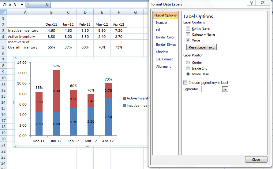
How-to Put Percentage Labels on Top of a Stacked Column Chart - Excel Dashboard Templates
Create Dynamic Chart Data Labels with Slicers - Excel Campus Step 6: Setup the Pivot Table and Slicer. The final step is to make the data labels interactive. We do this with a pivot table and slicer. The source data for the pivot table is the Table on the left side in the image below. This table contains the three options for the different data labels.

How to Add Data Labels in Excel - Excelchat | Excelchat
Apply Custom Data Labels to Charted Points - Peltier Tech Click once on a label to select the series of labels. Click again on a label to select just that specific label. Double click on the label to highlight the text of the label, or just click once to insert the cursor into the existing text. Type the text you want to display in the label, and press the Enter key.
How to add data labels from different column in an Excel chart?
adding extra data labels - Excel Help Forum add this data into the chart as a new series change the series type to be a line chart format the series to be on the secondary axis format the series to show the data labels format the series to have no markers and no line scale the secondary axis so the labels align with the tops of the bars/columns hide the secondary axis. Register To Reply

microsoft excel - Adding data label only to the last value - Super User
Using the CONCAT function to create custom data labels for an Excel ... Use the chart skittle (the "+" sign to the right of the chart) to select Data Labels and select More Options to display the Data Labels task pane. Check the Value From Cells checkbox and select the cells containing the custom labels, cells C5 to C16 in this example.
How to Add Data Labels in Excel - Excelchat | Excelchat
how to add data labels into Excel graphs - storytelling with data You can download the corresponding Excel file to follow along with these steps: Right-click on a point and choose Add Data Label. You can choose any point to add a label—I'm strategically choosing the endpoint because that's where a label would best align with my design. Excel defaults to labeling the numeric value, as shown below.
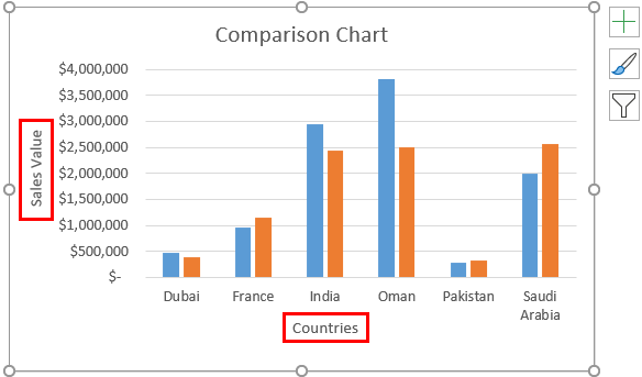
Comparison Chart in Excel | Adding Multiple Series Under Same Graph
Custom Chart Data Labels In Excel With Formulas - How To Excel At Excel Finally, in Column E, I used the CONCATENATE Function to join the sales figures from April 2016 and add the resultant percentage difference between April 2016 and the previous month's sales figures (from Column D).The result is the custom Excel data labels I need. The full formula used is in he screen grab below. You can check my blog posts for more information on CONCATENATE and here for ...

Enable or Disable Excel Data Labels at the click of a button - How To - PakAccountants.com
How to add data labels from different columns in an Excel chart? To add data labels, right-click the set of data in the chart, then pick the Add Data Labels option in Add Data Labels from the context menu. This will bring up a new window. Step 6 This is the data label that is currently shown in the chart. Step 7 If you click any data label, then all data labels will be selected.

Creating and editing a column chart - Bookboon
How to Customize Your Excel Pivot Chart Data Labels - dummies To add data labels, just select the command that corresponds to the location you want. To remove the labels, select the None command. If you want to specify what Excel should use for the data label, choose the More Data Labels Options command from the Data Labels menu. Excel displays the Format Data Labels pane.

30 How To Label Columns In Excel - Labels For You
Excel: Merge tables by matching column data or headers Select any cell within your main table and click the Merge Two Tables button on the Ablebits Data tab: Make sure the add-in got the range right, and click Next: Select the lookup table, and click Next: Specify the column pairs to match, Seller and Product in our case, and click Next: Tip.
November 2018

How to Create Multi-Category Chart in Excel - Excel Board
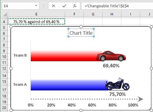
How to create dependent on a volume chart title - Microsoft Excel 2016
Quick Tip: Excel 2013 offers flexible data labels - TechRepublic
Post a Comment for "41 excel add data labels from different column"